Ranked batch-mode sampling
When querying from unlabeled data, sometimes you have the resources to label multiple instances at the same time. Classical uncertainty sampling however, does not quite support this scenario. To address this issue, multiple strategies were proposed, for instance Ranked batch-mode queries by Cardoso et al., which is implemented in modAL.
In this method, each example \(x\) is scored using the formula
where \(\alpha = \frac{|X_{unlabeled}|}{|X_{unlabeled}| + |X_{labeled}|}\), \(X_{labeled}\) is the labeled dataset, \(U(x)\) is the uncertainty of predictions for \(x\), and \(\Phi\) is a so-called similarity function, for instance cosine similarity. This latter function measures how well the feature space is explored near \(x\). (The lower the better.)
After scoring, the highest scored instance is put at the top of a list. The instance is removed from the pool and the score is recalculated until the desired amount of instances are selected.
In here, we will use the Iris dataset to demonstrate this. For more information on the iris dataset, see its wikipedia page or the documentation of its scikit-learn interface.
[1]:
import numpy as np
from sklearn.datasets import load_iris

# Loading the dataset
iris = load_iris()
X_raw = iris['data']
y_raw = iris['target']

# Isolate our examples for our labeled dataset.
n_labeled_examples = X_raw.shape[0]
training_indices = np.random.randint(low=0, high=len(X_raw)+1, size=3)

# Defining the training data
X_training = X_raw[training_indices]
y_training = y_raw[training_indices]

# Isolate the non-training examples we'll be querying.
X_pool = np.delete(X_raw, training_indices, axis=0)
y_pool = np.delete(y_raw, training_indices, axis=0)
For visualization purposes, we also perform a PCA transformation on the dataset.
[2]:
from sklearn.decomposition import PCA

# Define our PCA transformer and fit it onto our raw dataset.
pca = PCA(n_components=2)
pca.fit(X=X_raw)
[2]:
PCA(copy=True, iterated_power='auto', n_components=2, random_state=None,
  svd_solver='auto', tol=0.0, whiten=False)
Now we initialize an ActiveLearner.
[3]:
from modAL.models import ActiveLearner
from modAL.batch import uncertainty_batch_sampling
from sklearn.neighbors import KNeighborsClassifier

# Specify our core estimator.
knn = KNeighborsClassifier(n_neighbors=3)

learner = ActiveLearner(
    estimator=knn,
    query_strategy=uncertainty_batch_sampling,
    X_training=X_training, y_training=y_training
)
[4]:
from modAL.batch import ranked_batch
from modAL.uncertainty import classifier_uncertainty
from sklearn.metrics.pairwise import pairwise_distances

uncertainty = classifier_uncertainty(learner, X_pool)
distance_scores = pairwise_distances(X_pool, X_training, metric='euclidean').min(axis=1)
similarity_scores = 1 / (1 + distance_scores)

alpha = len(X_training)/len(X_raw)

scores = alpha * (1 - similarity_scores) + (1 - alpha) * uncertainty
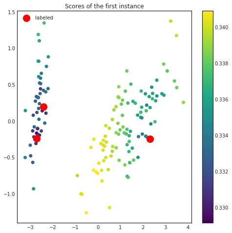
Now we can visualize the scores for the first instance during the first query.
[5]:
import matplotlib.pyplot as plt
%matplotlib inline
transformed_pool = pca.transform(X_pool)
transformed_training = pca.transform(X_training)

with plt.style.context('seaborn-white'):
    plt.figure(figsize=(8, 8))
    plt.scatter(transformed_pool[:, 0], transformed_pool[:, 1], c=scores, cmap='viridis')
    plt.colorbar()
    plt.scatter(transformed_training[:, 0], transformed_training[:, 1], c='r', s=200, label='labeled')
    plt.title('Scores of the first instance')
    plt.legend()
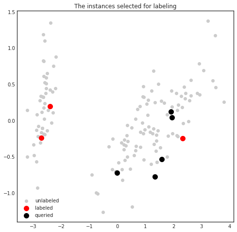
After the scores have been calculated, the highest scoring instance is selected and removed from the pool. This instance is not queried yet! The scores will be recalculated until the desired number of examples are available to send for query. In this setting, we shall visualize the instances to be queried in the first batch.
[6]:
query_idx, query_instances = learner.query(X_pool, n_instances=5)
[7]:
transformed_batch = pca.transform(query_instances)

with plt.style.context('seaborn-white'):
    plt.figure(figsize=(8, 8))
    plt.scatter(transformed_pool[:, 0], transformed_pool[:, 1], c='0.8', label='unlabeled')
    plt.scatter(transformed_training[:, 0], transformed_training[:, 1], c='r', s=100, label='labeled')
    plt.scatter(transformed_batch[:, 0], transformed_batch[:, 1], c='k', s=100, label='queried')
    plt.title('The instances selected for labeling')
    plt.legend()