Active regression
In this example, we are going to demonstrate how can the ActiveLearner be used for active regression using Gaussian processes. Since Gaussian processes provide a way to quantify uncertainty of the predictions as the covariance function of the process, they can be used in an active learning setting.
[1]:
import numpy as np
import matplotlib.pyplot as plt
from sklearn.gaussian_process import GaussianProcessRegressor
from sklearn.gaussian_process.kernels import WhiteKernel, RBF
from modAL.models import ActiveLearner

%matplotlib inline
The dataset
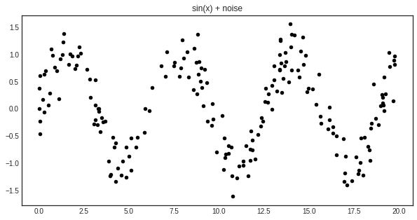
For this example, we shall try to learn the noisy sine function:
[2]:
X = np.random.choice(np.linspace(0, 20, 10000), size=200, replace=False).reshape(-1, 1)
y = np.sin(X) + np.random.normal(scale=0.3, size=X.shape)
[3]:
with plt.style.context('seaborn-white'):
    plt.figure(figsize=(10, 5))
    plt.scatter(X, y, c='k', s=20)
    plt.title('sin(x) + noise')
    plt.show()
Uncertainty measure and query strategy for Gaussian processes
For active learning, we shall define a custom query strategy tailored to Gaussian processes. More information on how to write your custom query strategies can be found at the page Extending modAL. In a nutshell, a query stategy in modAL is a function taking (at least) two arguments (an estimator object and a pool of examples), outputting the index of the queried instance and the instance itself. In our case, the arguments are
regressor and X.
[4]:
def GP_regression_std(regressor, X):
    _, std = regressor.predict(X, return_std=True)
    query_idx = np.argmax(std)
    return query_idx, X[query_idx]
Active learning
Initializing the active learner is as simple as always.
[5]:
n_initial = 5
initial_idx = np.random.choice(range(len(X)), size=n_initial, replace=False)
X_training, y_training = X[initial_idx], y[initial_idx]

kernel = RBF(length_scale=1.0, length_scale_bounds=(1e-2, 1e3)) \
         + WhiteKernel(noise_level=1, noise_level_bounds=(1e-10, 1e+1))

regressor = ActiveLearner(
    estimator=GaussianProcessRegressor(kernel=kernel),
    query_strategy=GP_regression_std,
    X_training=X_training.reshape(-1, 1), y_training=y_training.reshape(-1, 1)
)
The initial regressor is not very accurate.
[6]:
X_grid = np.linspace(0, 20, 1000)
y_pred, y_std = regressor.predict(X_grid.reshape(-1, 1), return_std=True)
y_pred, y_std = y_pred.ravel(), y_std.ravel()
[7]:
with plt.style.context('seaborn-white'):
    plt.figure(figsize=(10, 5))
    plt.plot(X_grid, y_pred)
    plt.fill_between(X_grid, y_pred - y_std, y_pred + y_std, alpha=0.2)
    plt.scatter(X, y, c='k', s=20)
    plt.title('Initial prediction')
    plt.show()
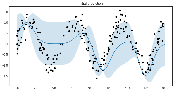
The blue band enveloping the regressor represents the standard deviation of the Gaussian process at the given point. Now we are ready to do active learning!
[8]:
n_queries = 10
for idx in range(n_queries):
    query_idx, query_instance = regressor.query(X)
    regressor.teach(X[query_idx].reshape(1, -1), y[query_idx].reshape(1, -1))
[9]:
y_pred_final, y_std_final = regressor.predict(X_grid.reshape(-1, 1), return_std=True)
y_pred_final, y_std_final = y_pred_final.ravel(), y_std_final.ravel()
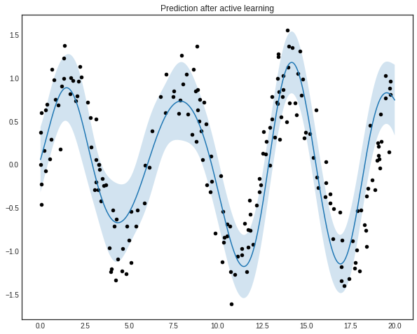
[10]:
with plt.style.context('seaborn-white'):
    plt.figure(figsize=(10, 8))
    plt.plot(X_grid, y_pred_final)
    plt.fill_between(X_grid, y_pred_final - y_std_final, y_pred_final + y_std_final, alpha=0.2)
    plt.scatter(X, y, c='k', s=20)
    plt.title('Prediction after active learning')
    plt.show()